![]()
![]()
![]()
holodeck allows quick and simple creation of simulated
multivariate data with variables that co-vary or discriminate between
levels of a categorical variable. The resulting simulated multivariate
dataframes are useful for testing the performance of multivariate
statistical techniques under different scenarios, power analysis, or
just doing a sanity check when trying out a new multivariate method.
From CRAN:
install.packages("holodeck)Development version from r-universe:
install.packages('holodeck', repos = c('https://aariq.r-universe.dev', 'https://cloud.r-project.org'))holodeck is built to work with dplyr
functions, including group_by() and the pipe
(%>%). purrr is helpful for iterating
simulated data. For these examples I’ll use ropls for PCA
and PLS-DA.
library(holodeck)
library(dplyr)
library(tibble)
library(purrr)
library(ropls)Let’s say we want to learn more about how principal component analysis (PCA) works. Specifically, what matters more in terms of creating a principal component—variance or covariance of variables? To this end, you might create a dataframe with a few variables with high covariance and low variance and another set of variables with low covariance and high variance
set.seed(925)
df1 <-
  sim_covar(n_obs = 20, n_vars = 5, cov = 0.9, var = 1, name = "high_cov") %>%
  sim_covar(n_vars = 5, cov = 0.1, var = 2, name = "high_var")
Explore covariance structure visually. The diagonal is variance.
df1 %>%
  cov() %>%
  heatmap(Rowv = NA, Colv = NA, symm = TRUE, margins = c(6,6), main = "Covariance")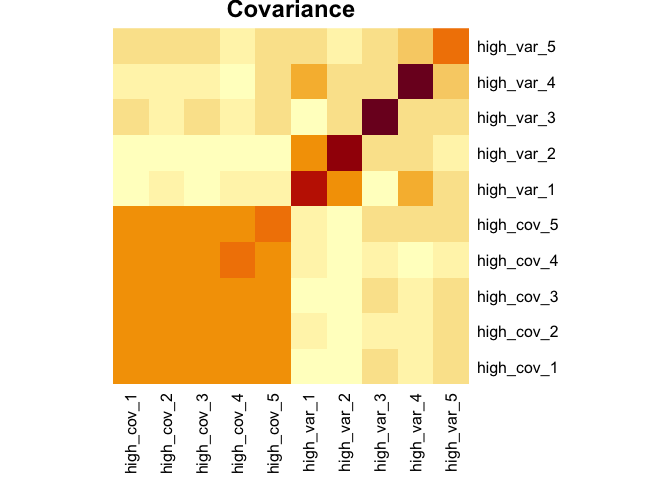
Now let’s make this dataset a little more complex. We can add a factor variable, some variables that discriminate between the levels of that factor, and add some missing values.
set.seed(501)
df2 <-
  df1 %>%
  sim_cat(n_groups = 3, name = "factor") %>%
  group_by(factor) %>%
  sim_discr(n_vars = 5, var = 1, cov = 0, group_means = c(-1.3, 0, 1.3), name = "discr") %>%
  sim_discr(n_vars = 5, var = 1, cov = 0, group_means = c(0, 0.5, 1), name = "discr2") %>%
  sim_missing(prop = 0.1) %>%
  ungroup()
df2
#> # A tibble: 20 × 21
#>    factor high_cov_1 high_cov_2 high_cov_3 high_cov_4 high_cov_5 high_var_1
#>    <chr>       <dbl>      <dbl>      <dbl>      <dbl>      <dbl>      <dbl>
#>  1 a           0.472   -0.362       0.253      0.281      NA        -0.0873
#>  2 a          -1.50    -1.65       -1.47      -1.93       NA        NA
#>  3 a           1.13    NA          NA          1.41        0.345     0.871
#>  4 a           0.982    0.740       1.16       1.14        0.866    NA
#>  5 a          -0.773   NA          NA         -1.21       -1.25     -1.53
#>  6 a           0.302    0.130      -0.309      0.0725      0.725     0.890
#>  7 a          -0.117    0.00163     0.0596    -0.542      -0.269    NA
#>  8 b           2.16     2.47        1.38       1.62        1.62     -2.43
#>  9 b          NA       -0.509      -0.529     -0.842      -1.04      1.25
#> 10 b           0.609    0.195       0.720      0.930       0.595    -0.562
#> 11 b           1.81     1.15        1.43       1.09        1.39     -0.934
#> 12 b           0.954    0.234       0.247      0.248       0.751     1.95
#> 13 b          -1.03    NA          -1.70      -1.27       -1.64      0.670
#> 14 b          NA        0.380       0.177     NA           0.550     2.68
#> 15 c          -0.214   -0.390      -0.476     -0.878      -0.328     0.665
#> 16 c           0.827    0.556       0.620      0.491       0.814    -0.0121
#> 17 c          -0.399   -0.862      -0.385     -0.935      -0.802    NA
#> 18 c          -1.09    -1.32       -0.720     -1.88       -1.76     -2.05
#> 19 c          -0.181   -0.155      -0.774      0.0395     -0.770     1.81
#> 20 c           0.882   NA           0.758      1.24       NA         1.11
#> # ℹ 14 more variables: high_var_2 <dbl>, high_var_3 <dbl>, high_var_4 <dbl>,
#> #   high_var_5 <dbl>, discr_1 <dbl>, discr_2 <dbl>, discr_3 <dbl>,
#> #   discr_4 <dbl>, discr_5 <dbl>, discr2_1 <dbl>, discr2_2 <dbl>,
#> # discr2_3 <dbl>, discr2_4 <dbl>, discr2_5 <dbl>pca <- opls(select(df2, -factor), fig.pdfC = "none", info.txtC = "none")
plot(pca, parAsColFcVn = df2$factor, typeVc = "x-score")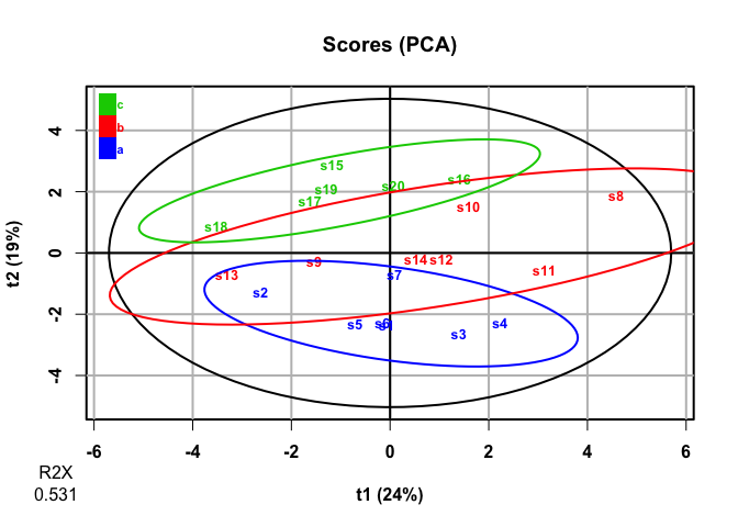
getLoadingMN(pca) %>%
  as_tibble(rownames = "variable") %>%
  arrange(desc(abs(p1)))
#> # A tibble: 20 × 4
#>    variable         p1      p2       p3
#>    <chr>         <dbl>   <dbl>    <dbl>
#>  1 high_cov_2  0.415    0.0534  0.0137
#>  2 high_cov_1  0.407    0.0383  0.0208
#>  3 high_cov_5  0.401    0.0163  0.104
#>  4 high_cov_3  0.400    0.0301 -0.0837
#>  5 high_cov_4  0.387    0.0218  0.00556
#>  6 discr_5    -0.224    0.262  -0.136
#>  7 high_var_2 -0.195    0.0848  0.240
#>  8 discr2_1    0.167    0.396  -0.167
#>  9 discr_2    -0.163    0.322  -0.202
#> 10 high_var_5  0.115   -0.132   0.261
#> 11 discr2_5    0.0967   0.267   0.114
#> 12 high_var_1 -0.0930  -0.0102  0.457
#> 13 discr2_4    0.0834   0.308   0.0924
#> 14 discr_3    -0.0627   0.376  -0.0152
#> 15 discr2_2   -0.0412   0.138   0.539
#> 16 discr_1    -0.0407   0.319   0.0471
#> 17 discr2_3   -0.0394   0.176  -0.358
#> 18 discr_4     0.0363   0.400   0.144
#> 19 high_var_3 -0.0101  -0.0629  0.0483
#> 20 high_var_4 -0.00471  0.131   0.308
It looks like PCA mostly picks up on the variables with high
covariance, not the variables that discriminate among
levels of factor. This makes sense, as PCA is an
unsupervised analysis.
plsda <- opls(select(df2, -factor), df2$factor, predI = 2, permI = 10, fig.pdfC = "none", info.txtC = "none")

plot(plsda, typeVc = "x-score")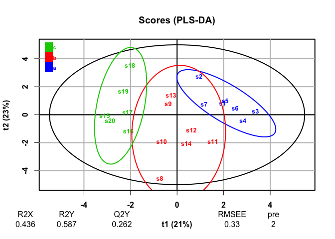
getVipVn(plsda) %>%
  tibble::enframe(name = "variable", value = "VIP") %>%
  arrange(desc(VIP))
#> # A tibble: 20 × 2
#>    variable      VIP
#>    <chr>       <dbl>
#>  1 discr_4    1.54
#>  2 discr_1    1.48
#>  3 discr_2    1.47
#>  4 discr_5    1.44
#>  5 discr_3    1.42
#>  6 discr2_1   1.31
#>  7 discr2_4   1.09
#>  8 high_cov_2 1.08
#>  9 discr2_3   0.996
#> 10 high_cov_1 0.944
#> 11 discr2_2   0.884
#> 12 high_cov_5 0.790
#> 13 discr2_5   0.650
#> 14 high_var_5 0.639
#> 15 high_var_2 0.582
#> 16 high_cov_4 0.530
#> 17 high_cov_3 0.423
#> 18 high_var_4 0.358
#> 19 high_var_1 0.200
#> 20 high_var_3 0.0860
PLS-DA, a supervised analysis, finds discrimination among groups and finds that the discriminating variables we generated are most responsible for those differences.