Using variational techniques we address some epidemiological problems as the incidence curve decomposition or the estimation of the functional relationship between epidemiological indicators. We also propose a learning method for the short time forecast of the trend incidence curve.
EpiInvert
: an incidence curve decomposition by inverting the renewal
equation.
EpiInvertForecastEpiIndicators
: estimation of the delay and ratio between epidemiological
indicators.
We also present in Rt Comparison a comparative analysis of the methods : EpiInvert, EpiEstim, Wallinga-Teunis and EpiNow2.
You can install the development version of EpiInvert from GitHub with:
 install.packages("devtools")
devtools::install_github("lalvarezmat/EpiInvert")We attach some required packages
library(EpiInvert)
library(ggplot2)
library(dplyr)
library(grid)
Loading data on COVID-19 daily incidence up to 2022-05-05 for France, Germany, the USA and the UK:
data(incidence)
tail(incidence)
#>           date   FRA    DEU    USA    UK
#> 828 2022-04-30 49482  11718  23349     0
#> 829 2022-05-01 36726   4032  16153     0
#> 830 2022-05-02  8737 113522  81644    32
#> 831 2022-05-03 67017 106631  61743 35518
#> 832 2022-05-04 47925  96167 114308 16924
#> 833 2022-05-05 44225  85073  72158 12460
Loading some festive days for the same countries:
data(festives)
head(festives)
#>          USA        DEU        FRA         UK
#> 1 2020-01-01 2020-01-01 2020-01-01 2020-01-01
#> 2 2020-01-20 2020-04-10 2020-04-10 2020-04-10
#> 3 2020-02-17 2020-04-13 2020-04-13 2020-04-13
#> 4 2020-05-25 2020-05-01 2020-05-01 2020-05-08
#> 5 2020-06-21 2020-05-21 2020-05-08 2020-05-25
#> 6 2020-07-03 2020-06-01 2020-05-21 2020-06-21
Executing EpiInvert using Germany data:
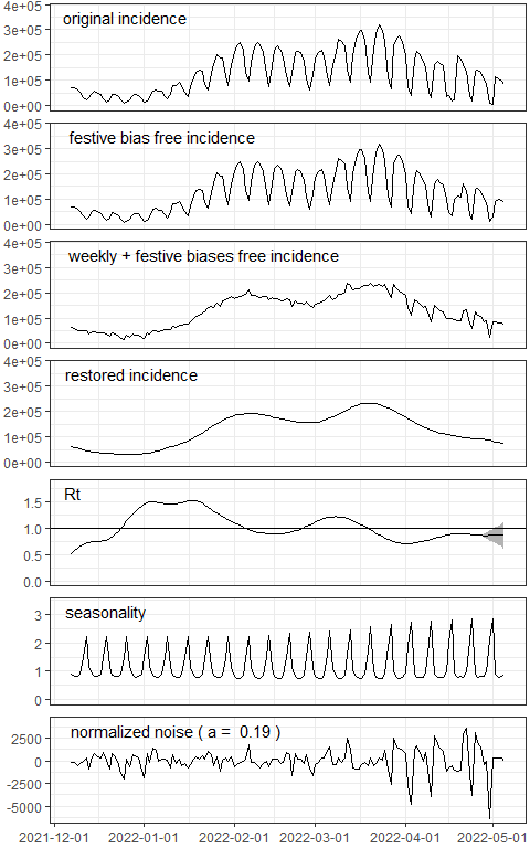
res <- EpiInvert(incidence$DEU,"2022-05-05",festives$DEU)Plotting the results:
EpiInvert_plot(res)
For a detailed description of EpiInvert outcomes see the EpiInvert vignette.